The mathematics of Sagefy

In this article, I’m going to talk about some of the mathematical models I’m using in Sagefy so far. I’m going to discuss some of the problems I’ve run into, and what problems are still ahead. I’m hoping to occasionally update this article as the math that Sagefy uses changes.

What is Sagefy?

Sagefy is an open-content adaptive learning system. Open-content means anyone can create and update learning content, like Wikipedia. Adaptive learning means the content changes based on the learner’s goal and their prior knowledge. The combination means anyone can learn just about anything, regardless of their prior knowledge. To learn more about Sagefy, check out this in-depth article.

The Sagefy Learner Experience

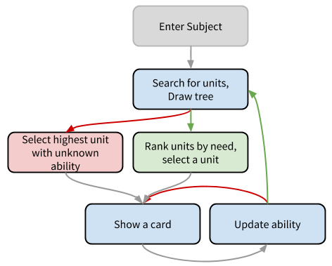
After you create an account, the first thing to do is to find a subject. A subject is like a course or a collection of courses. You can think of it like folders on your computer; they nest. You add the subject to your list of subjects. Then, when you start the subject, you’ll see a tree of units. Each unit is a single learning objective. Then, Sagefy will ask you to choose which unit you’d like to start with. Sagefy presents a recommended unit based on what you know. After choosing a unit, Sagefy will show you a card. A card is a single learning activity, like a video or multiple choice question. As you use the cards, Sagefy updates it’s model of how much you know the unit. When you’ve learned the unit, you choose another. The trio of subject, unit, and card define the learning experience.

$The flow of the Sagefy learner experience.$

Popular Models of Learning

There’s a few different learning models out there. The subject is diverse. “Building Intelligent Interactive Tutors” by Beverly Park Woolf is a more comprehensive treatment. Here’s some of the major ones:

Forgetting Curve

The Ebbinghaus Forgetting Curve is one of the oldest models. Depending on the strength of the memory, our ability to remember generally follows this formula:

$The Ebbinghaus Forgetting Curve, r = e^(-t/s)$

In this formula, r is retention, tau is time, and s is the strength of the memory.

Learning Curve

The opposite of the forgetting curve is the learning curve:

$The Learning Curve, a = 1-e^(-t/s)$

Where a is learning. Some authors suggest an alternative model for learning, a sigmoid function:

$Alternative learning curve, a = 1/(1+e^(-(t-u)/s)))$

Bayesian Knowledge Tracing

Bayesian Knowledge Tracing determines how likely a learner knows a skill, based on the learner’s responses.

Bayesian Knowledge Tracing derives from Bayes’ Theorem.

![Bayes’ Theorem, p(A

B) = p(A) * p(B

A) / p(B)](/images/math-5.png)

We call…

p(A|B) the posterior — what we believe after seeing the data.
p(A) the prior — what we believe before the data.
p(B|A) the likelihood —given our prior belief, how likely was the data.
p(B) the normalizer — how likely is the data given all hypotheses.

p(B) is often difficult to formulate. We can use this as a replacement:

![A Bayes normalizer. p(B) = p(A) * p(B

A) + p(~A) * p(B

~A)](/images/math-6.png)

~ in this case means not.

For BKT, we have the follow factors:

p(L) — probability the learner learned the skill.
p(C) — probability the learner will get the item correct.
p(T) — probability the learner will learn the skill on a particular item.
p(G) — probability the learner will guess the right answer.
p(S) — probability the learner will mess up even knowing the skill.

For any item, the probability of getting the answer correct is:

$Probability of a correct answer: p(C) = p(L) * p(~S) + p(~L) * p(G)$

Putting this all together, the probability the learner has learned the skill is, given a correct answer:

$The probability the learner has learned the skill, given a correct answer.$

Given an incorrect answer:

$The probability the learner has learned the skill, given an incorrect answer.$

We also must account for the idea the learner may have improved the skill during the card. So…

$We now include transit, as the probability the learner has learned the action during the action.$

The power of Bayes is the ability to update the model each time we receive new information. We don’t have to operate on larger data sets at less frequent intervals. We can constantly update the model just a little bit each time.

For a better explanation, I recommend this video from Ryan Baker’s Big Data and Education course.

Item Response Theory

Item Response Theory determines how likely a learner will correctly answer a particular question. It is a logistic function. We use IRT is more commonly in testing, but we can use IRT in adaptive learning as well. The parameters read:

theta — learner ability.
b — item difficulty.
a — item discrimination; how likely the item determines ability.
c — item guess.

There are two common formulations:

$The simpler IRT, which only uses item difficulty.$ $The more complex IRT, which uses difficulty, discrimination, and guess.$

The formulas change slightly depending on author.

We can extend Item Response Theory into Performance Factors Analysis. PFA is a competing model with Bayesian Knowledge Tracing.

Knowledge Space Theory

Knowledge Space Theory represents what skills learner knows. KST derives from antimatroids.

We assume a learner has either learned a skill or not. Given skills +, -, *, and /, we would form prerequisites, such as:

+ -> -
+ -> *
* -> /

The knowledge space represents all possible sets of knowledge a learner might have, such as:

none
+
+, -
+, *
+, *, /
+, -, *, /

An individual learner has a likelihood for each of these sets. KST makes the assumption that an individual question may inquire about multiple skills. We begin by asking questions that use multiple skills, and work backwards to assess learner knowledge.

Several automated systems exist to automatically determine prerequisites based on learner performance.

Spaced Repetition

Spaced Repetition suggests that learners should spread out their practice. Reviews should happen less frequently as ability improves.

The most popular algorithm is SuperMemo 2. The first review is after 1 day, the second review is after 6 days. After which, the next review is:

$SuperMemo 2. i(n) = i(n-1) * e$

…where e is how difficult or easy the item is. e is between 1.3 and 2.5, and it uses learner responses on a Likert scale to determine the next time to review.

Later versions of SuperMemo include other considerations, such as:

Similar cards
Previous iteration duration
Ebbinghaus forgetting curve

The latest is version 11/15.

Why Sagefy uses Bayesian Knowledge Tracing

Sagefy uses Bayesian Knowledge Tracing. The reason is that it is a simple formula and computationally inexpensive. The other advantage is that with Bayes, the model updates each time the learner interacts with the system a little bit each time. This feature avoids expensive modeling computations all at once. That means that Sagefy can both scale more easily and handle a larger diversity of content.

Adding Time to Bayesian Knowledge Tracing

Bayesian Knowledge Tracing does not consider forgetting. To account for forgetting, I have added a taste of the Ebbinghaus forgetting curve into the final calculation. A new formula which calculates belief, which is our confidence in p(L) given the elapsed time:

exp(-1 * time_delta * (1 — learned) / belief_factor)

I set my belief factor to 708000 based on guess-and-check. Likely, I could optimize this value later on.

How I’m Working to Learn Card, Unit, and Subject Parameters

Everything here so far lays out how to estimate how likely the learner knows the unit. But, what the other parameters, and how do we come to know those? This is the more challenging area.

Parameters of Cards, Units, and Subjects

Cards. In Bayesian Knowledge Tracing, most implementations assign a Guess, Slip, and Transit at the unit level. But, for Sagefy, to get deeper information, I’ve assigned those parameters to cards. Transit informs us of the quality of the card. Guess and Slip informs us of the difficulty of the card. Difficulty helps us to choose cards appropriate to the learner’s ability. We also want to track the number of learners who will we will impact when we make changes to the card.

Units. We want to know a way of determining approximately how much time or how many cards it takes on average to learn the unit. This is the difficulty of the unit. We can judge the quality of the unit based on the average ability of the learners of the unit. We also want to track the number of learners who will we will impact when we make changes to the unit.

Subjects. We want to know a way of informing the learner how much time it will take to complete the subject, given their currency state of progress. This is the difficulty of the subject. We can calculate the difficulty of the subject by summing up the difficulty of the remaining units. We can also calculate quality in a similar fashion, but using a mean instead of a sum. We also want to track the number of learners who will we will impact when we make changes to the subject.

You can see we have lots of data about the smallest entities, and less data about higher entities. We track fine data about cards, a little less about units, and subjects just aggregate unit data. So for this section of the article, the focus will be on card parameters.

Probability Mass Functions

Bayes gives us the ability to make constant updates to our models instead of making big and heavy calculations all at once. To achieve this, we work with distributions. So instead of just resulting with a number, we have a line chart. On one axis is the possible values, on the other axis is the probability of that value being the correct answer. So as we get more data, the graph tightens around a single value.

There’s two types of distributions. One is continuous. In a continuous distribution, we have a single equation that represents the entire graph. The other is discrete. So we have specific data points that represent our graph. Computers naturally can work with discrete much more quickly than continuous. The official name of a discrete distribution is the probability mass function. Because Sagefy is ultimately made of servers, the PMF is the more efficient and easier to use choice.

PMFs are easy to work with in Bayes. Each possible value gets its own update that matches the p(A|B) = p(A) * p(B|A) / p(B) formula. Then we normalize the PMF after the update so that the sum probability of the values is 1. With the PMF, the normalizer takes care of p(B). And we already have p(A) which is the previous set of hypotheses. That means we need a way to compute p(B|A), the likelihood.

Everything I know about probability mass functions I learned from the book Think Bayes by Allen Downey. He gives a much better explanation than I could, and the book is free.

Card Parameters

We need to update Guess, Slip, and Transit per learner response. Guess should increase with correct answers and decrease with incorrect answers. Slip should increase with incorrect answers and decrease with correct answers. Transit should increase if the later responses are more correct, and decrease if the later responses are less correct.

For Guess and Slip, I figured how how to calculate the likelihood, though it doesn’t work as accurately as I’d like. The formula for if a learner will get an answer correct is:

learned * (1-slip) + (1-learned) * guess

and incorrect…

learned * slip + (1-learned) * (1-guess)

If the learner got it right, I can use the first formula as the likelihood. If the learner got it wrong, I can use the second formula. Learned is the learner’s learned. You take the prior slip to calculate guess, and the prior guess to calculate slip. The value of guess or slip is just each hypothesis (so you do this calculation per each hypothetical value). Doing the math, it means earlier learners will impact guess more, and later learners will impact slip more as expected.

When I ran this in simulation, it held a strong correlation to the initial values. But, they were off by scale. I have manually adjusted the scale in Sagefy. Transit is likely at play at throwing off these calculations, but I was unable to find a formula to take out this factor automatically. This is an opportunity for improvement.

I was unable to find a way to calculate a likelihood for transit. I know the following is true:

transit = (learned_post — learned_pre) / (1 — learned_pre)

This likelihood never panned out in simulation, so for now Sagefy has a set transit for all cards. This is a major opportunity for improvement.

I haven’t figured out how how to calculate the number of learners quite yet. That’s more of a technical challenge than a mathematical one.

Unit and Subject Parameters

I haven’t done the work to calculate the two unit and two subject parameters: difficulty and number of learners. These are both essentially database queries. The responses table can inform the difficulty. Learners subscribe to subjects, and not units. The solution requires figuring out all the relationships and then counting from there. Not impossible, but not easy either.

How I’m Simulating Models and Error Rates

Because Sagefy is new, I don’t have much real user data to test my model against. For now, I’m using simulated data. I created a script that will create a random collection of subjects, units, cards, and users, all of each with random parameters within ranges. I’m using triangle ranges instead of completely linear randomization to more closely simulate real data. Then, I can run my model against the simulated data, and take error rates. We can calculate the error rate for each parameter as:

$Error rate. sqrt( sum( (si — ri) ^ 2 ) / n )$

Where s_i is the simulated value (each example), r_i is the real value, n is the number of examples.

When I modeled this, I was able to see my errors shrink by changing the number of steps in my PMF. I also saw improvements by scaling down guess and slip… again, that’s still a mystery at this point. Hopefully, if Sagefy attracts users, we will be able to create better models using real data instead of simulated data.

Traversing the Graph of Units

Bayesian Knowledge Tracing helps us within a unit. But, subjects contain many units. To work with the course, we must iterate over the graph of units.

We collect the subject of units that the learner will be participating in. We will need to diagnose any units which the learner hasn’t seen. We will also need to diagnose any units that the learner viewed, but we are no longer confident in the ability score due to time.

The following is an example of this process, known as a graph traversal.

$An example graph of units.$

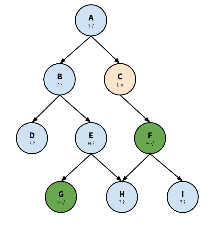
The algorithm makes use of depth first search. We start near the end of the tree, and walk our way down as we diagnose. We record each node in one of three lists: Diagnose, Ready, and Learned.

First, we start at node “A”. We diagnose an L (low score). Because it is a low score, we will continue to traverse the tree. Append “A” to list Diagnose.

Next, we will continue to node “C”. This is because we have higher confidence in “C” than “B”. “C” is already diagnosed. Append “C” to list Ready. We note that “C” has one dependency, “A”.

Third, we continue to node “F” (depth-first search). We are confident that the learner knows node “F”, and we start on the other side of the chain. Append “F” to Learned. Although “F” requires “I”, because we are confident in high ability for “F”, we will not diagnose “I”.

Because “C” has no other requires, we go back to “B”. We find it is a low ability. Append to Ready, 1 dependent: A.

We know more about “E” than “D”, so we continue to “E”. We find “E” is a low ability. Append to Ready, 2 dependents: A and B.

We already know “G”, so append “G” to Learned.

We diagnose “H”, and find it is low ability. Append to Ready, 3 dependents: “A”, “B”, and “E”. If the learner hadn’t learned “F”, unit “H” would have 4 dependencies instead of 3. The algorithm considers how many nodes depend on the given node, rather than how deep in the graph the node is.

Finally, we diagnose node “D” with low ability. Append to Ready, and there are 2 dependents: “A” and “B”.

$Now, our graph of units after diagnosis.$

We also have the following lists:

Diagnose: [] Ready: [A, C, B, E, H, D] Learned: [F, G]

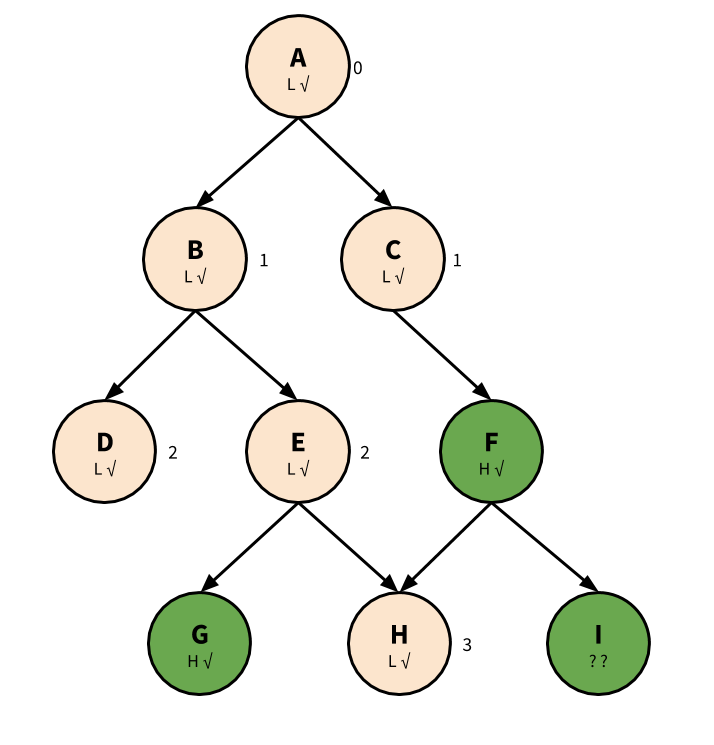
We are now ready to starting the learning process.

The following is overly simplistic; most learners will not ‘learn’ a unit in their first attempt at it. If at any time the unit composition changes, when we come back to the tree, we will need to diagnose any new units. Additionally, learners will need to review some units every now-and-again to keep the confidence scores up.

In the ready list, A, B, and E have requires, so those are not options to the learner yet. The available ready nodes are C, D, and H.

“H” has the most dependents, so Sagefy would recommend “H” as the starting place for the learner. Let’s say, though, the learner choose to learn unit “D” first.

Now the remaining set is C and H. The learner chooses H. So now the remaining set is E and C. Let’s say the learner chooses C.

Now, the only option remaining is E. After E, the learner would do B, then A.

Choosing Cards

After the learner selects a unit, then Sagefy must choose a card for them. Several factors come into play:

How well has the learner mastered this unit? p(L)
Which cards are assessment v non-assessment cards? (e.g. Videos are non-assessment, multiple choice is assessment)
Has the learner recently seen the card?
Does the card require another card first?
How good is the card? p(T)

Our goals are as follows:

We want to show cards of appropriate difficulty. A card with high slip would not be appropriate for someone with a low p(L), for example.
We want to focus on non-assessment cards for low p(L), and assessment cards for a high p(L).
We want to avoid showing a card the learner has seen recently, when possible.
We want to ‘follow’ card requires.

The current process works like this:

Find p(L).
Choose ten random cards in the unit.
Split up the cards by assessment versus non-assessment.
If the learner has a low p(L), be more likely to prefer non-assessment. As p(L) increases, prefer assessment.
For an assessment card, try to find one where the probability of correct is greater than 0.25 and less than 0.75. Otherwise, show any assessment card.
For non-assessment, just pick the first one.
Otherwise, choose any remaining card available.

A few things could improve here. We can add tags, track how the learner does with different kinds of cards, and use p(T) to choose better quality cards. Overall, this is not as difficult of a problem as figuring out what the learner does and does not know.

Contributor Experience

The contributor experience is still a work in progress.

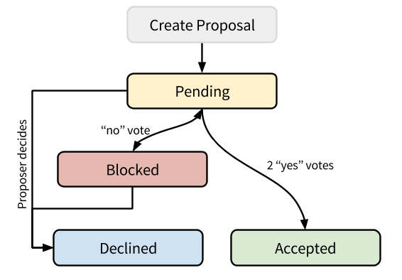
In most open-content systems, anyone can edit. But, usually there’s a number of people subscribed to all changes to the content. When a change occurs that was not discussed, the change is immediately reverted. Only by discussion and consent is the change made permanent.

Sagefy codifies this process by not allowing direct edits, but by allowing anyone to propose changes to content. Then, other users can vote on the proposal. With enough approving votes, Sagefy makes the change. Sagefy keeps a record of all the changes too. With any significant dissent, Sagefy blocks the proposal.

Contributor Ratings and Consensus-Based Decision Making

$The proposal flow.$

The decision to accept a proposal has a few factors: the reputation of the proposer and voters and the usage of the entity.

Entity Calculation

We calculate the “Yes” vote power as the sum of the proposer and the “yes” voters’ vote power.

We calculate the “No” vote power as the sum of the “no” voters’ vote power.

To accept a proposal, the proposal requires log2(number_of_learners) in “yes” vote power.

To block a proposal, the proposal requires log100(number_of_learners) in “no” vote power.

To unblock a proposal, we must work together to reduce the “no” vote power to below this amount. Otherwise, the proposer can decline their proposal.

The reason for this is simple: its likely impossible to meet perfect consensus all the time. Yet, we should strongly consider dissent. Majority rule isn’t as powerful as near-consensus.

Example:

- Number of Learners, To Accept, To Block - 1, 0, 0 - 10, 3.32, 0.5 - 100, 6.64, 1 - 1000, 9.97, 1.5 - 10000, 13.28, 2 - 100000, 16.61, 2.5

Contributor Calculation

Each proposal and vote for a proposal in accepted state counts as +1 point. Sagefy calculates the vote power as 1-e^(-points/40). This may seem like a convoluted formula. The reason is to avoid “superusers” who by their linear reputation alone can make any change. The difference between 0 and 10 successful contributions gives us lots of information. 10 to 100, less so. And 100 to 1000, even less. We learn the most from the earliest examples, and less with each example.